CS 180 Project 2: Fun with Filters and Frequencies

Introduction

This project explores various techniques for processing and combining images using frequency-based methods. We delve into image sharpening by emphasizing high frequencies, edge extraction using finite difference kernels, and the creation of hybrid images by combining high and low frequencies from different sources. Additionally, we experiment with image blending at various frequencies using Gaussian and Laplacian stacks.

Part 1: Fun with Filters!

1.1 Finite Difference Operator

In this section, we apply finite difference operators to extract edge information from images. We begin by computing the partial derivatives in both x and y directions using simple finite difference kernels:

For x-direction: $$D_x = [-1, 1]$$
For y-direction: $$D_y = [-1, 1]^T$$

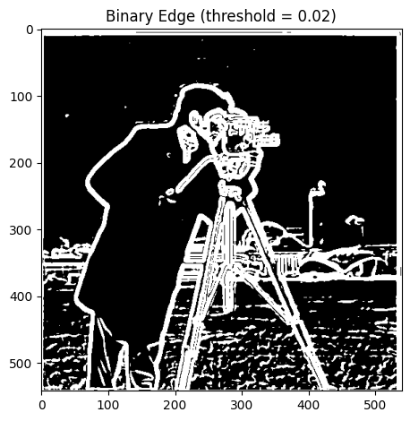
We convolve these operators with our image to obtain the discrete partial derivatives ∂I/∂x and ∂I/∂y. The gradient magnitude is then calculated as:

$$\nabla I = \sqrt{(\frac{\partial I}{\partial x})^2 + (\frac{\partial I}{\partial y})^2}$$

1.2 Derivative of Gaussian (DoG) Filter

However, these basic finite difference operators are highly sensitive to noise, resulting in discrete-looking edges. To mitigate this, we introduce Gaussian smoothing before gradient computation. We apply a 10x10 Gaussian kernel with σ = 2 to the image before computing the gradient. To reduce noise sensitivity in edge detection, we implement the Derivative of Gaussian (DoG) filter. This approach combines Gaussian smoothing with edge detection in a single operation. This Gaussian pre-filtering results in significantly smoother edge detection compared to the non-Gaussian version. The detected edges appear more continuous and less affected by small-scale noise.

We can achieve the same result more efficiently by convolving the Gaussian kernel with our difference operators first, then applying these combined kernels to the image. This approach, leveraging the commutative property of convolution, saves us an expensive image-wide convolution operation while producing identical results.

Part 2: Fun with Frequencies

2.1 Image "Sharpening"

Image sharpening is achieved by separating an image into its low and high frequency components, then enhancing the high frequency details. This process involves the following steps:

1. Apply a Gaussian filter to the original image to obtain the low frequency component.
2. Subtract the low frequency (Gaussian filtered) image from the original to isolate the high frequency details.
3. Add an amplified version of these high frequency details back to the original image.

The mathematical formula for this sharpening process can be expressed as:

$$I_{sharpened} = (α + 1) * I - α * (I * G)$$

Where:

• I is the original image
• G is the Gaussian kernel
• α is a parameter controlling the degree of sharpening
• * denotes convolution

We applied this sharpening technique to images of two iconic Indian monuments: the Taj Mahal and the Qutb Minar. The results demonstrate how this process can enhance the visibility of fine details:

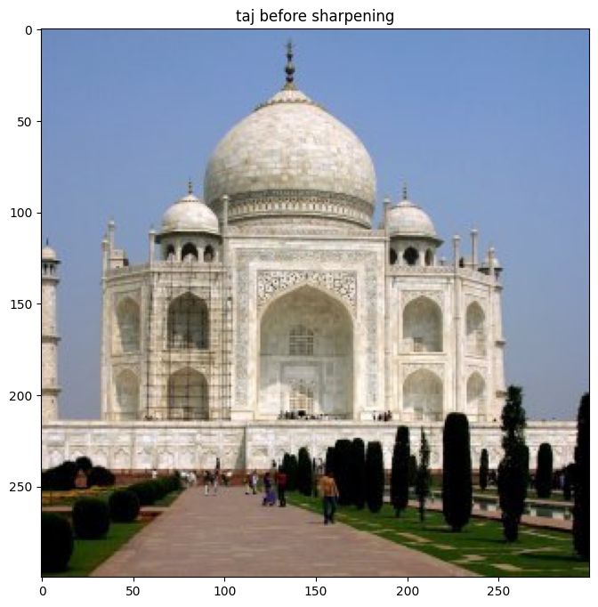
Original Taj Mahal

Sharpened Taj Mahal

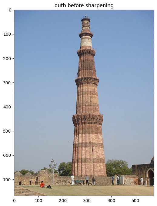
Original Qutb Minar

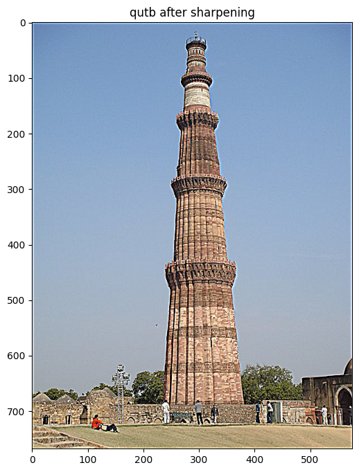
Sharpened Qutb Minar

As we can observe, the sharpening process significantly enhances the visibility of intricate details on both monuments. The architectural features, carvings, and textures become more prominent, allowing for a clearer appreciation of the craftsmanship involved in these historical structures.

2.2 Hybrid Images

Hybrid images are created by combining low frequencies from one image with high frequencies from another. This results in an image that appears different when viewed from near and far distances.

To create a hybrid image, we follow these steps:

1. Extract high frequencies from one image by subtracting a Gaussian-filtered version from the original.
2. Extract low frequencies from another image by applying a Gaussian filter.
3. Combine these two frequency components into a single image.

Example: Dog and Cat Hybrid

For this example, we created a hybrid image using a dog (low frequency) and a cat (high frequency). Before combining the images, we applied some preprocessing to align them better, including rotation and translation of the cat image.

We then applied low-pass and high-pass filters to the dog and cat images respectively, using Gaussian kernels with different sigma values to control the cutoff frequencies.

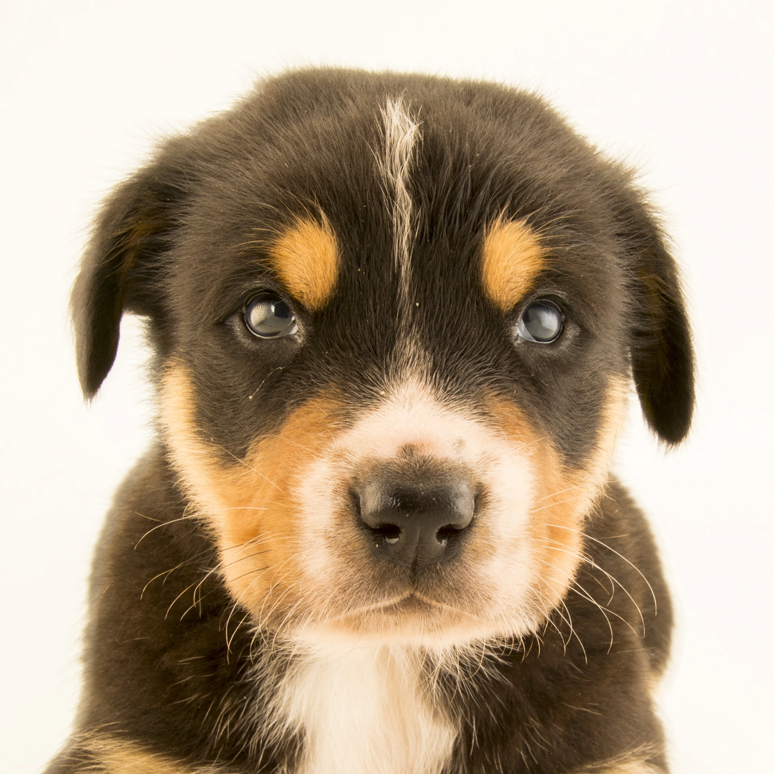
Original Dog Image

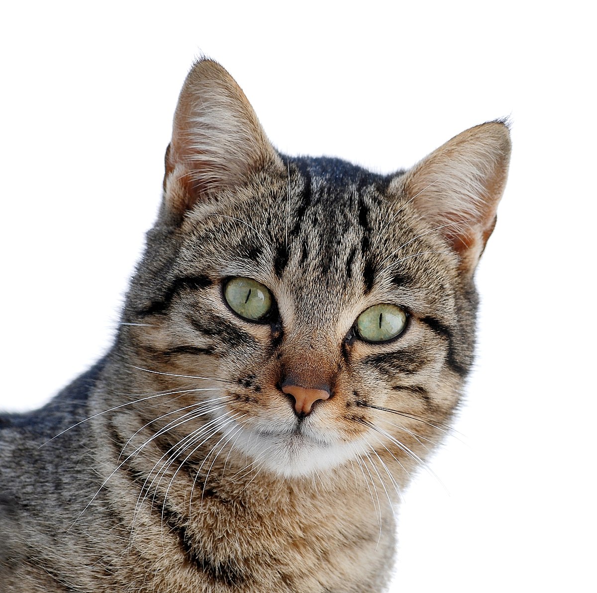
Original Cat Image

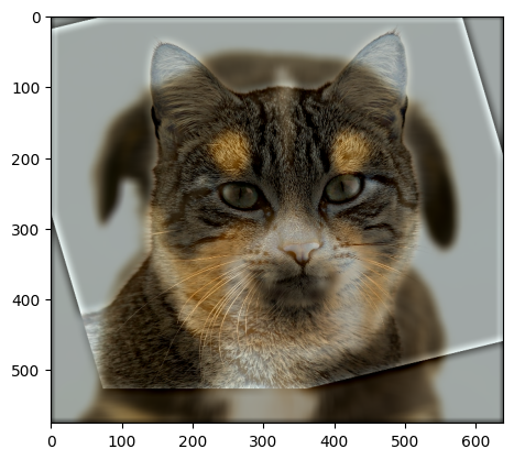
Hybrid Image

Interpreting the FFTs

We also visualized the Fourier transforms of the original images and the hybrid components:

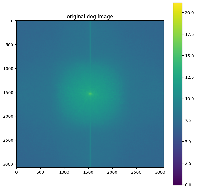
Dog Image FFT

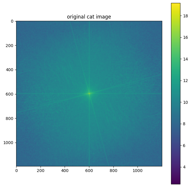
Cat Image FFT

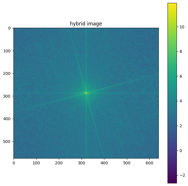
Hybrid Image FFT

Interpreting these FFTs:

• The dog image FFT shows more energy concentrated in the center, indicating dominant low frequencies.
• The cat image FFT has more energy spread out, representing higher frequency details.
• The hybrid image FFT combines both characteristics: a bright center (from the dog) and spread-out energy (from the cat).

This frequency domain representation explains why the hybrid image appears different at various distances. When viewed up close, the high-frequency details of the cat are visible. From a distance, these high frequencies become less perceptible, and the low-frequency structure of the dog dominates our perception.

The hybrid image technique demonstrates how our visual system processes different spatial frequencies and how this processing changes with viewing distance. It's a fascinating example of how understanding and manipulating frequency components can create intriguing visual effects.

Here are some more examples of hybrid images created using different image pairs:

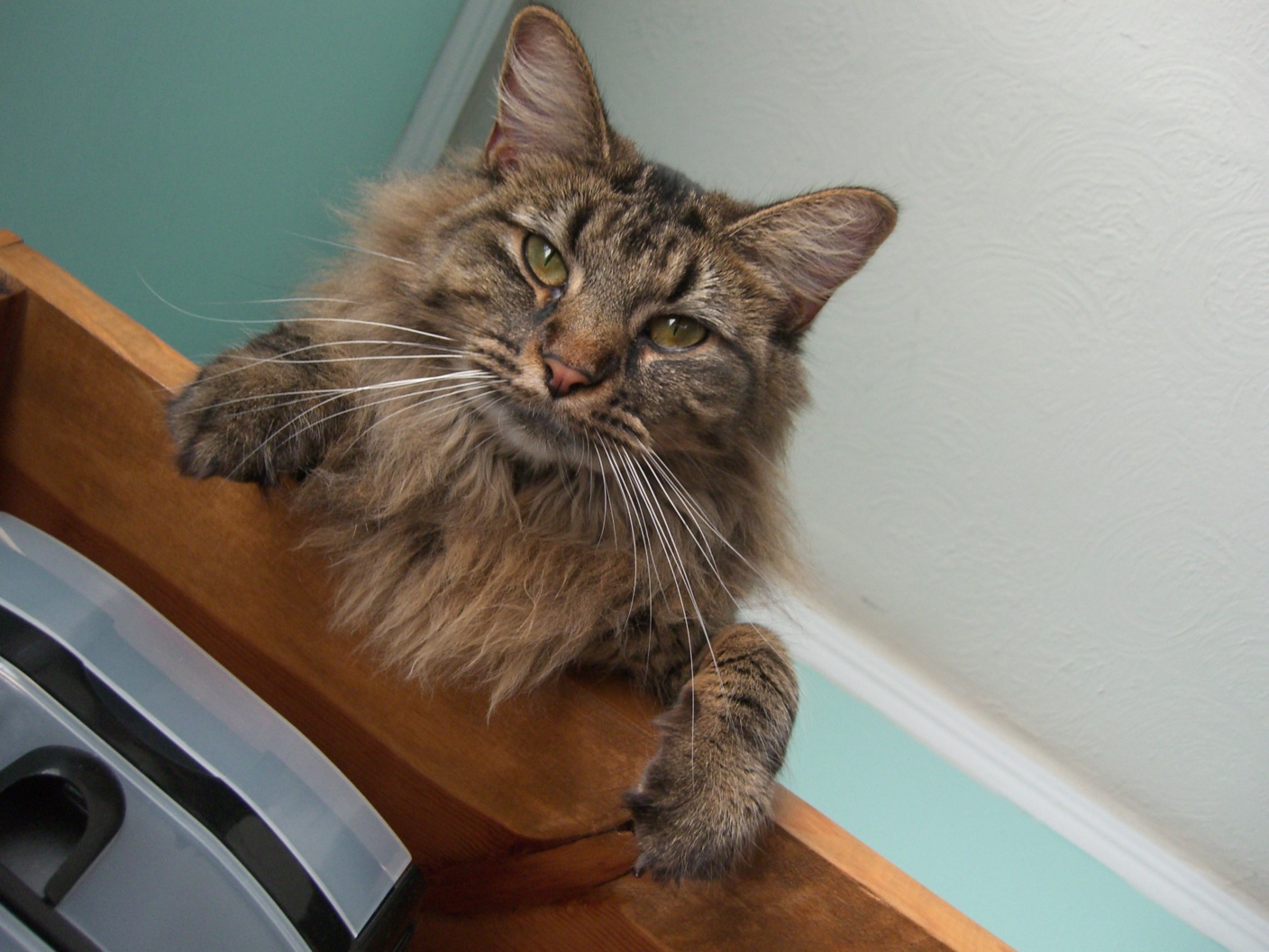
Original Nutmeg Image

Original Derek Image

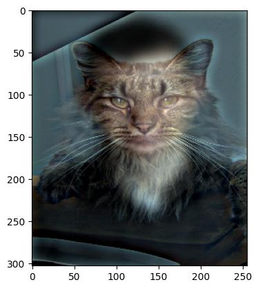
Hybrid Image

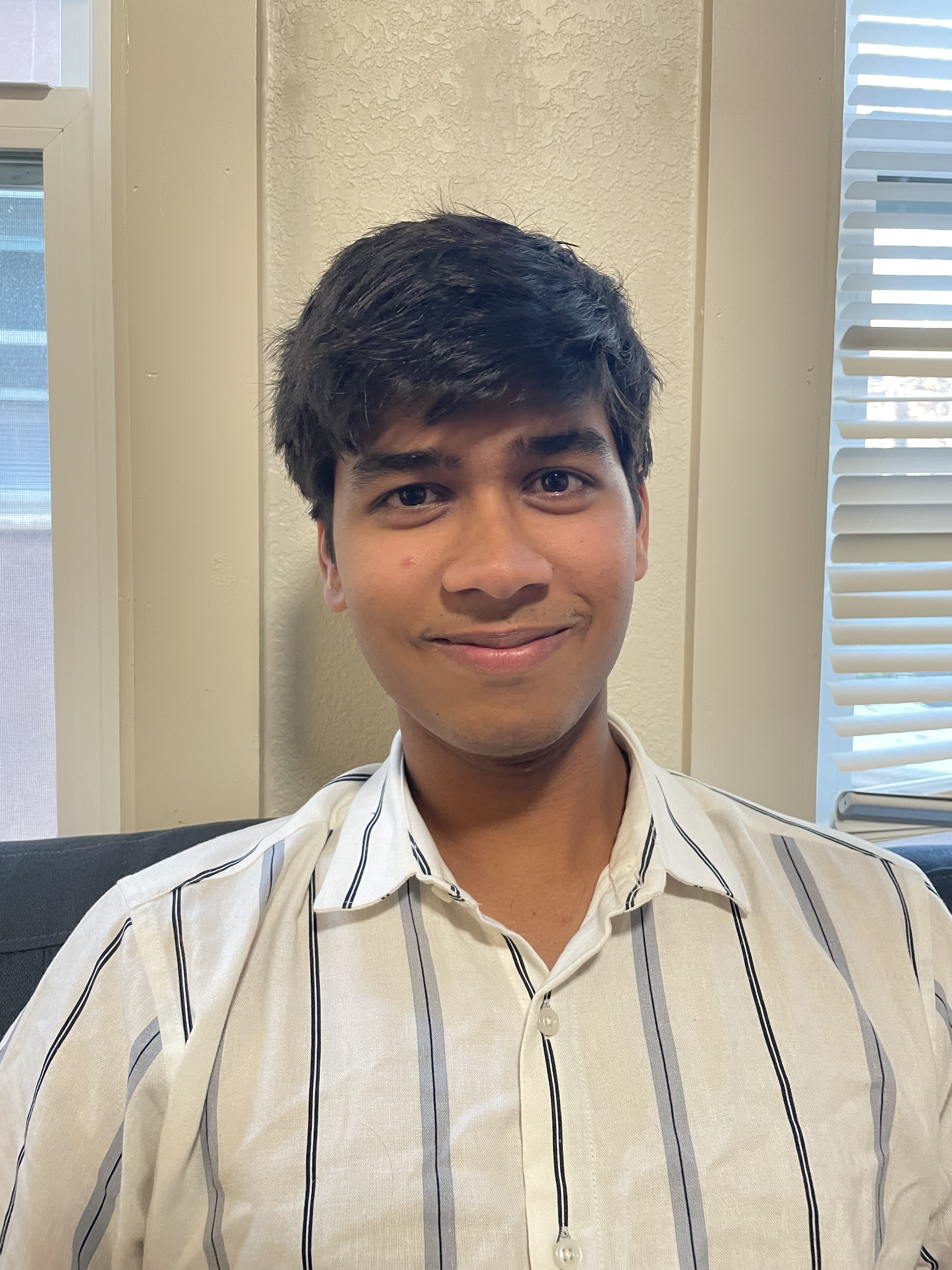
Original Arnav Smiling Image

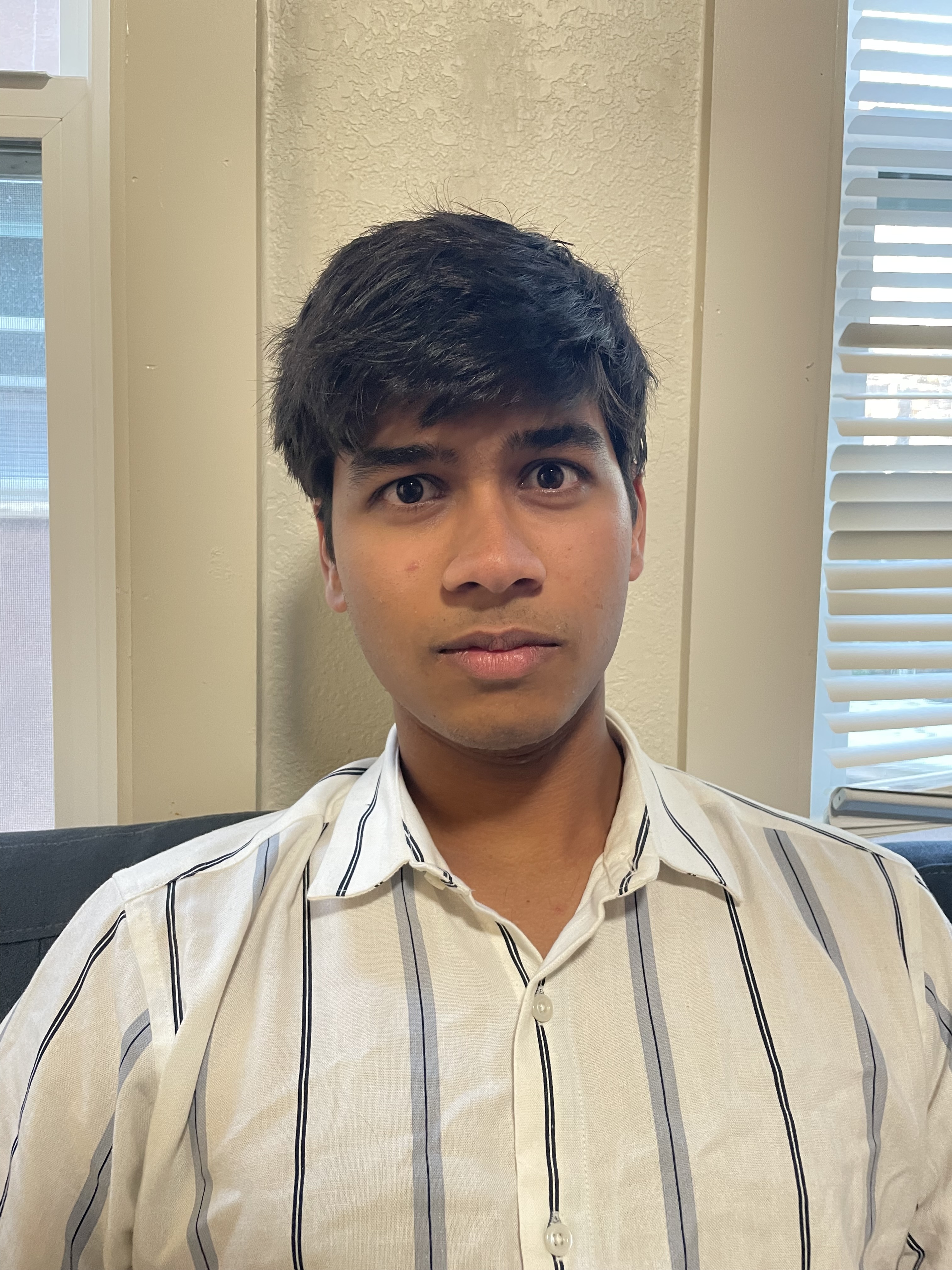
Original Arnav Serious Image

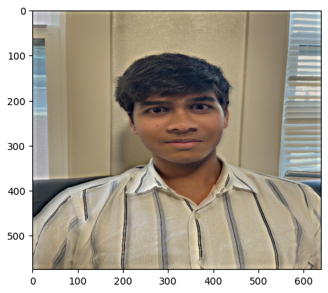
Hybrid Image

2.3 Gaussian and Laplacian Stacks

Now we move on to the problem of image blending. It's important to note that we're working with stacks rather than pyramids, so there's no downsampling of pixels involved. Instead, the downsampling effect in the stack is induced by increasing the sigma value for the Gaussian kernel.

The Gaussian stack is created by applying the Gaussian kernel with increasing values of sigma to the same image. For our implementation, we used 5 levels, with sigma values doubling at each level (2^i for i from 0 to 4).

Laplacian stacks are generated by differencing consecutive Gaussian filtered images: Lap[i] = Gauss[i+1] - Gauss[i].

We applied this method to both the apple and orange images to prepare for the blending process. Below are the visualizations of the Laplacian and Gaussian stacks for both images:

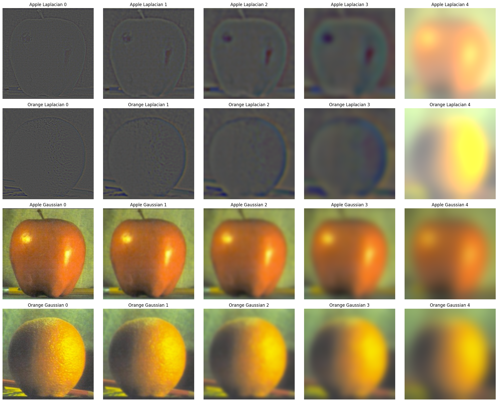
Apple and Orange Laplacian and Gaussian Stack

In these visualizations, each column represents a different level of the stack, from the finest details (left) to the coarsest (right). For the Laplacian stacks, we've added a constant (0.4) and clipped the values to [0, 1] for better visualization, as Laplacian images often contain both positive and negative values.

These stacks form the foundation for our multi-resolution blending technique, which we'll explore in the next section.

2.4 Multi-resolution Blending

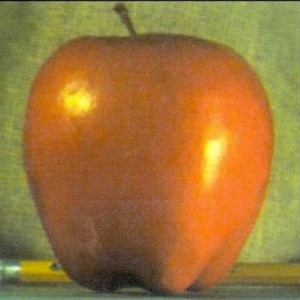
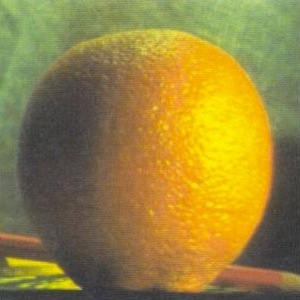
Building upon our Gaussian and Laplacian stacks, we now implement multi-resolution blending to seamlessly combine images. This technique allows us to blend images at different frequency levels, resulting in smooth transitions between the source images.

Our blending process involves the following steps:

1. Create Gaussian and Laplacian stacks for both input images
2. Generate a mask and its Gaussian stack
3. Blend the Laplacian stacks using the Gaussian mask stack
4. Reconstruct the final blended image by collapsing the blended Laplacian stack

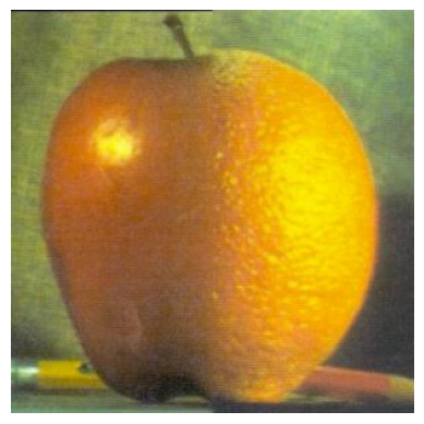
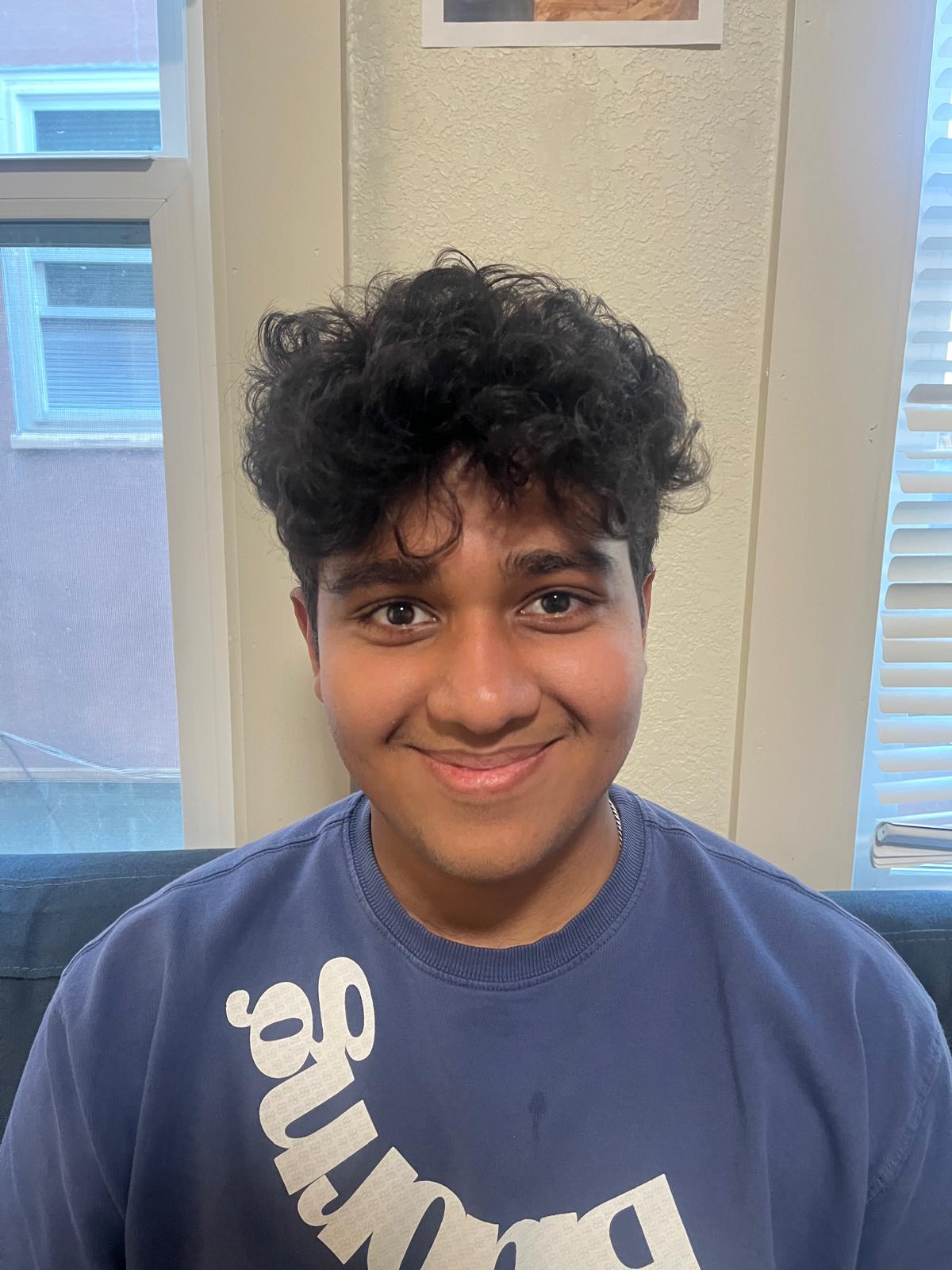
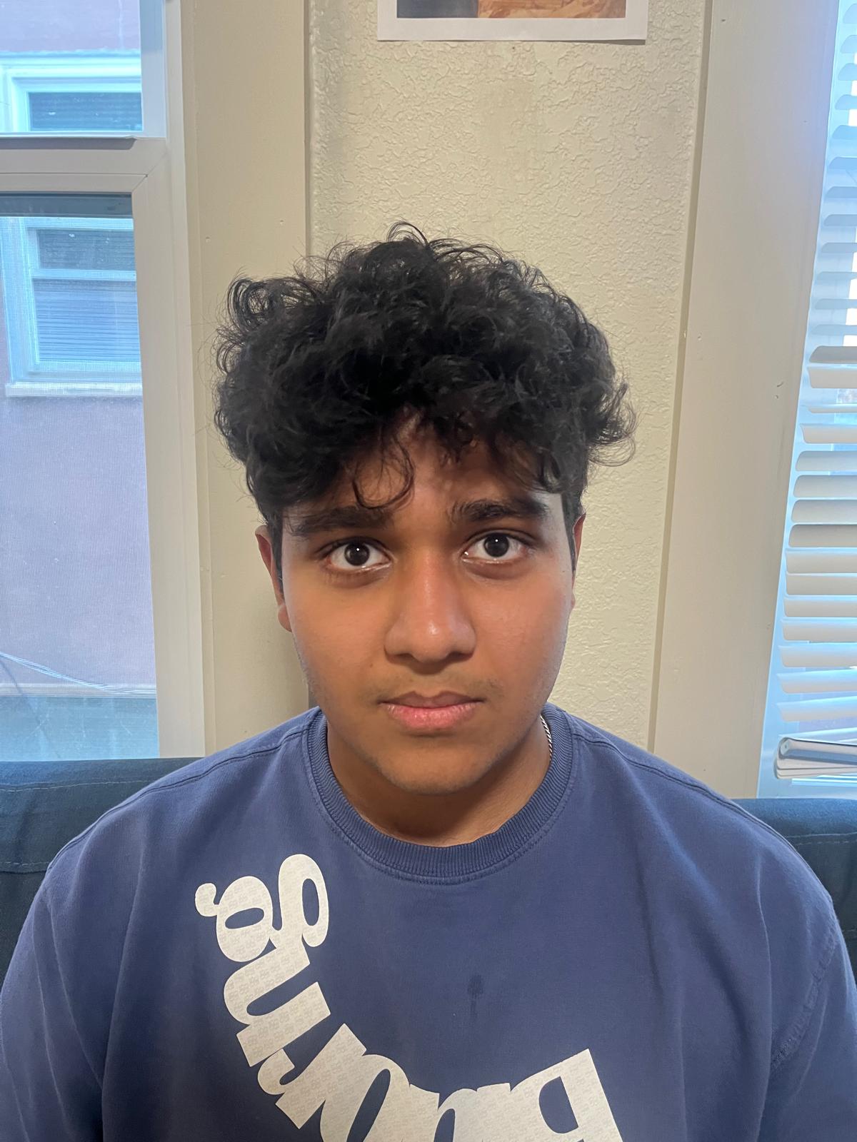
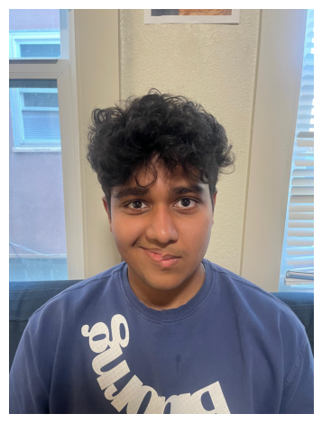
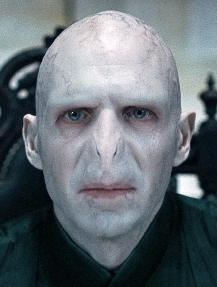
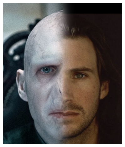
We applied this blending technique to several image pairs, using both even (vertical split) and uneven masks:

1. Apple and Orange (Classic Example)

2. Smiley Rhythm and Serious Rhythm

3. Voldemort and Ralph Fiennes

4. Girlfriend and Mango (Uneven Mask)

As a special treat for my girlfriend who loves mangoes, I created a unique blend using an uneven mask:

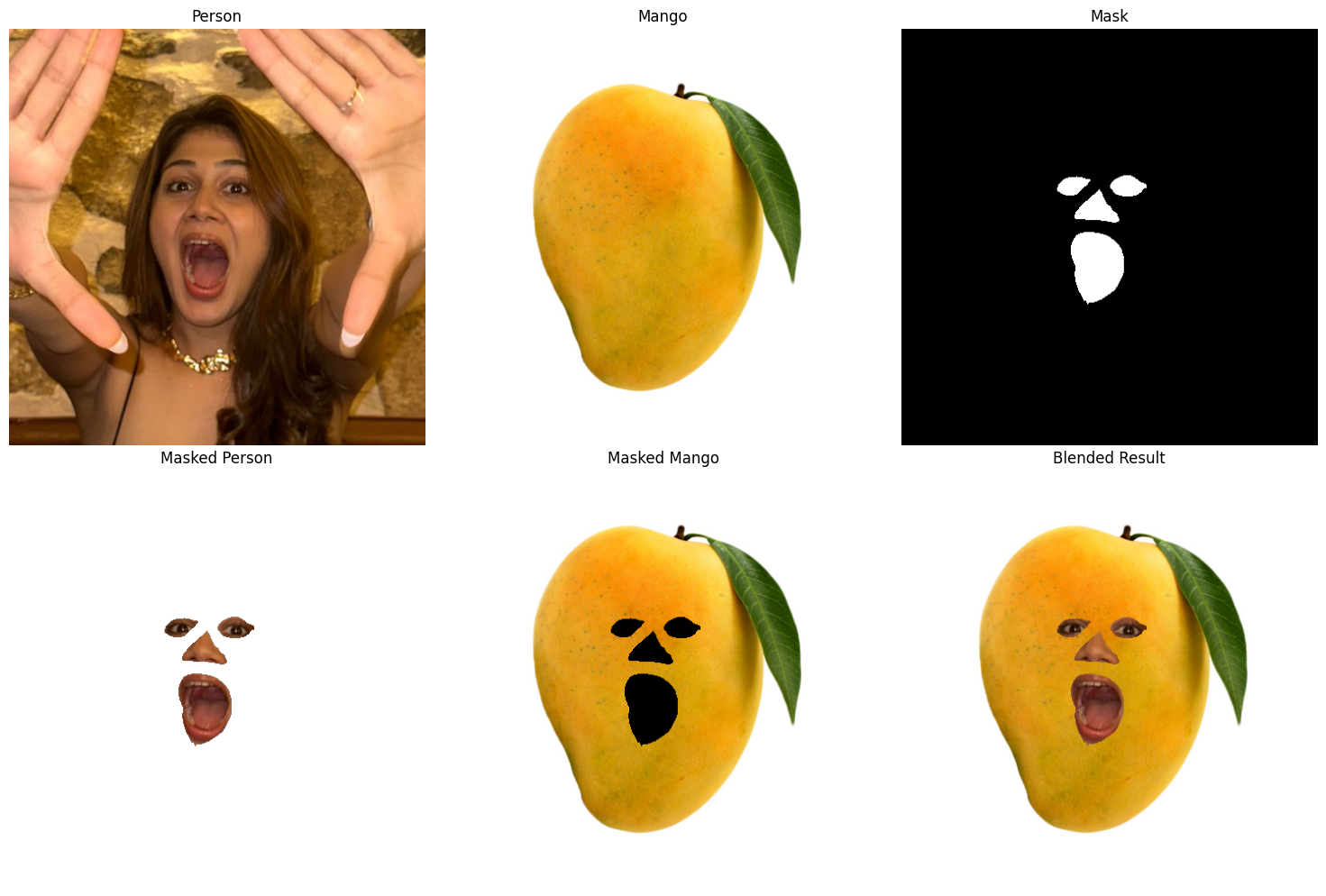
For this last example, I created a custom, uneven mask using an iPad to achieve a more artistic and personalized blend. The result showcases how multi-resolution blending can create seamless transitions even with complex, non-linear boundaries between images.

These examples demonstrate the versatility of multi-resolution blending in creating visually intriguing composites. The technique effectively combines images at various frequency levels, resulting in smooth transitions that maintain the detailed features of both source images.

Conclusion

This project has been an enlightening journey into the world of image processing, particularly in the realm of multi-resolution blending and frequency-based image manipulation. Through the process of implementing these techniques, I've gained several valuable insights:

1. The importance of trial and error in image processing cannot be overstated. What works well for one image pair might not be optimal for another, necessitating constant experimentation with parameters and techniques.
2. A solid understanding of the underlying mathematics is crucial. Knowing what a particular convolution or frequency manipulation will do to an image can significantly speed up the otherwise long and tenuous process of achieving desired results.
3. The value of visualizing intermediate steps. Examining Gaussian and Laplacian stacks, as well as frequency domain representations, provided invaluable insights into the workings of these algorithms.

This project has deepened my appreciation for the complexity and artistry involved in image processing. It has shown me that while computational techniques can achieve remarkable results, there's often a need for human intuition and creativity in guiding these processes to achieve the best outcomes.

In conclusion, this project has not only enhanced my technical skills in image processing but has also fostered a deeper appreciation for the interplay between mathematical theory, computational techniques, and creative problem-solving in the field of computer vision.