CS 180 Project 4: Image Warping and Mosaicing
By Rhythm Seth
Overview
This project explores image mosaicing techniques, including recovering homographies, warping images, and blending them into a seamless mosaic. We'll go through several steps to achieve these fascinating visual effects.
Part 1A: Recover Homographies
This function uses point correspondences to set up and solve a linear system, recovering the 3x3 homography matrix. We used more than 4 correspondences and implemented a least-squares solution for stability.
Where (x, y) are the coordinates in the first image, and (x', y') are the corresponding coordinates in the second image. This system of equations is then solved to find the entries of the homography matrix H.
Part 2: Warp the Images
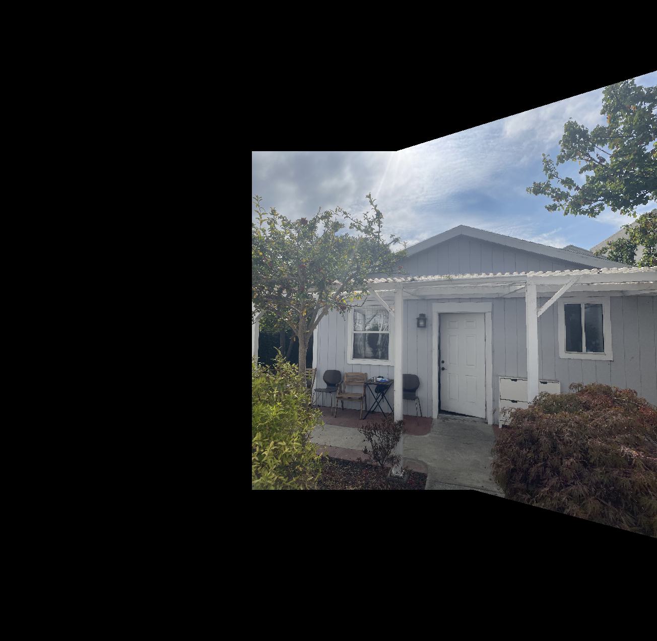
Using the computed homography, we implemented an image warping function. This function transforms the source image to align with the target image's perspective.
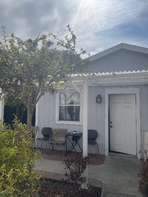
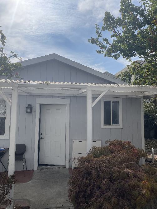
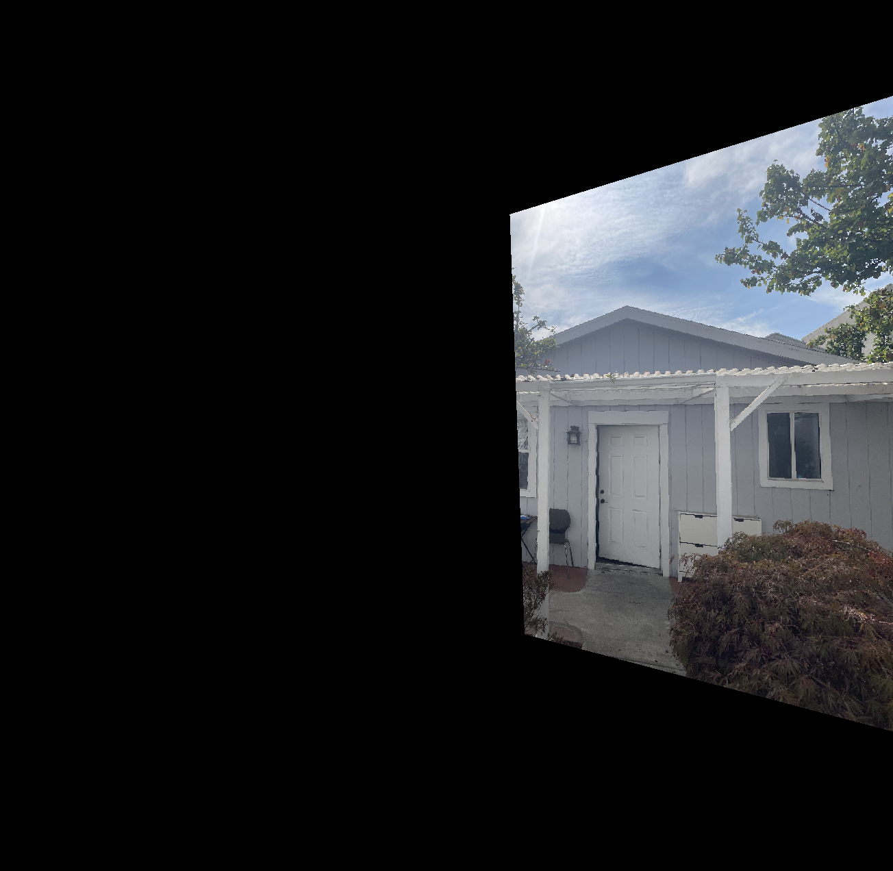
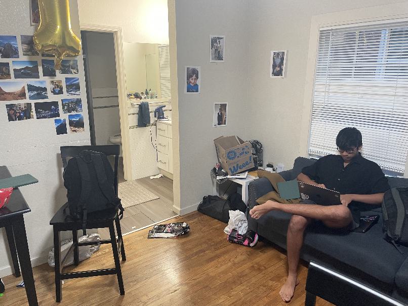
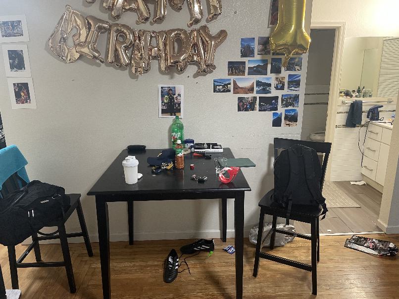
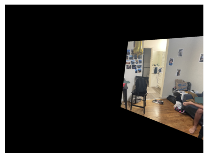
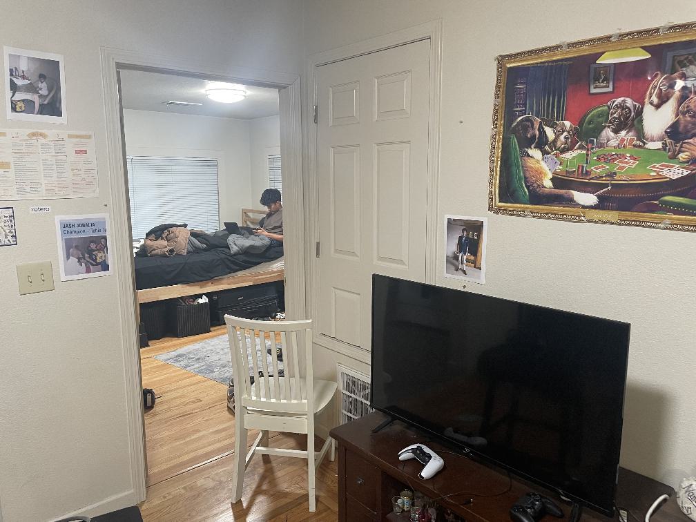
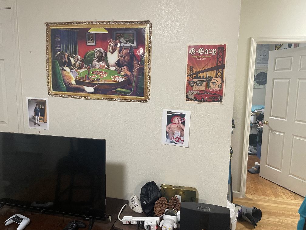
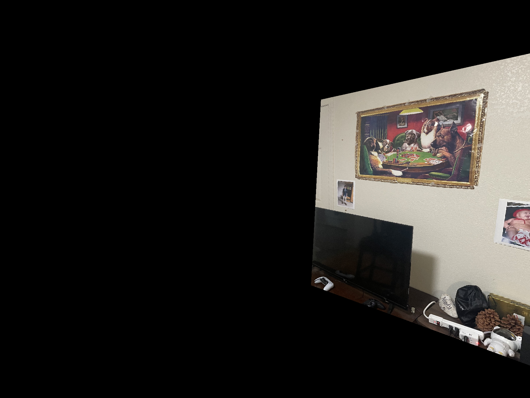
The warping process involves inverse mapping and interpolation to ensure smooth transformation of the image.
Part 3: Rectification
We demonstrated the rectification process by selecting a rectangular object in an image (painting) and warping it to an approximate rectangle. We used the provided online correspondence tool same as we did in Project 3. This technique is useful for correcting perspective distortions.
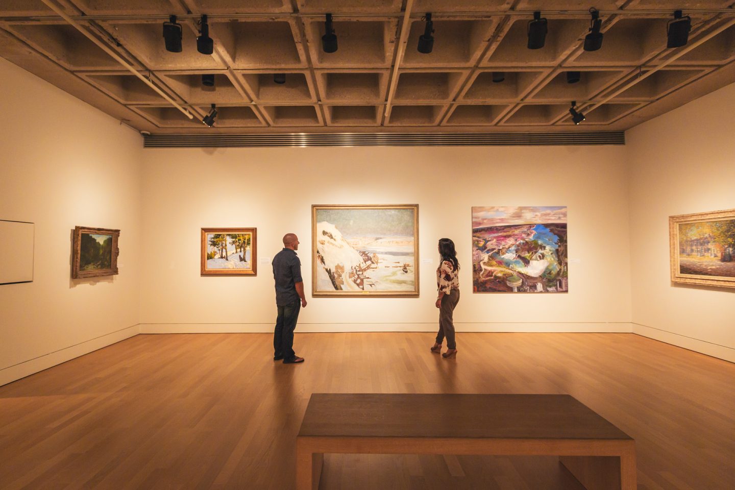
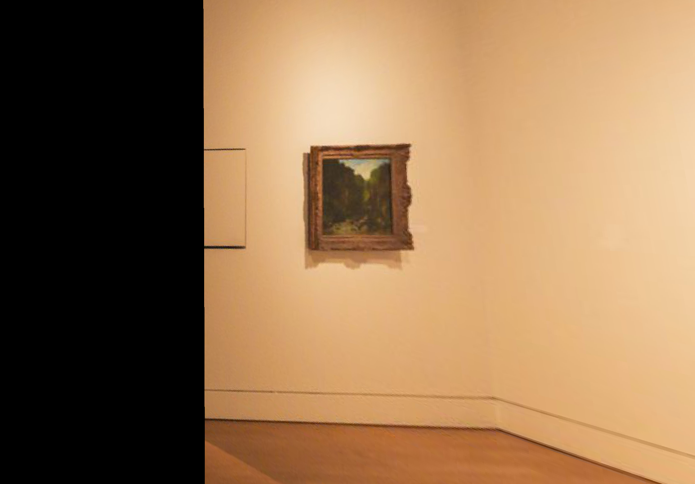
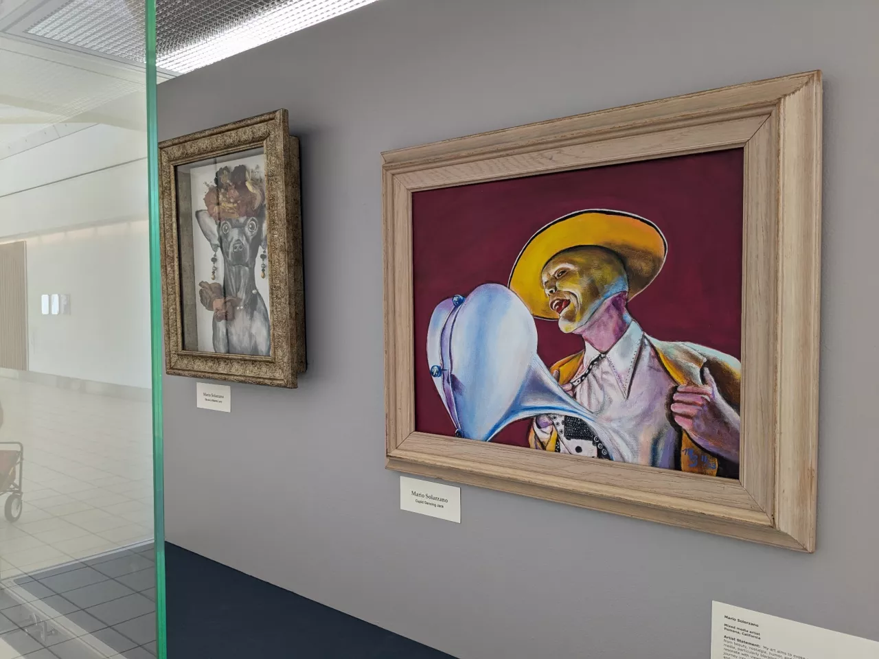
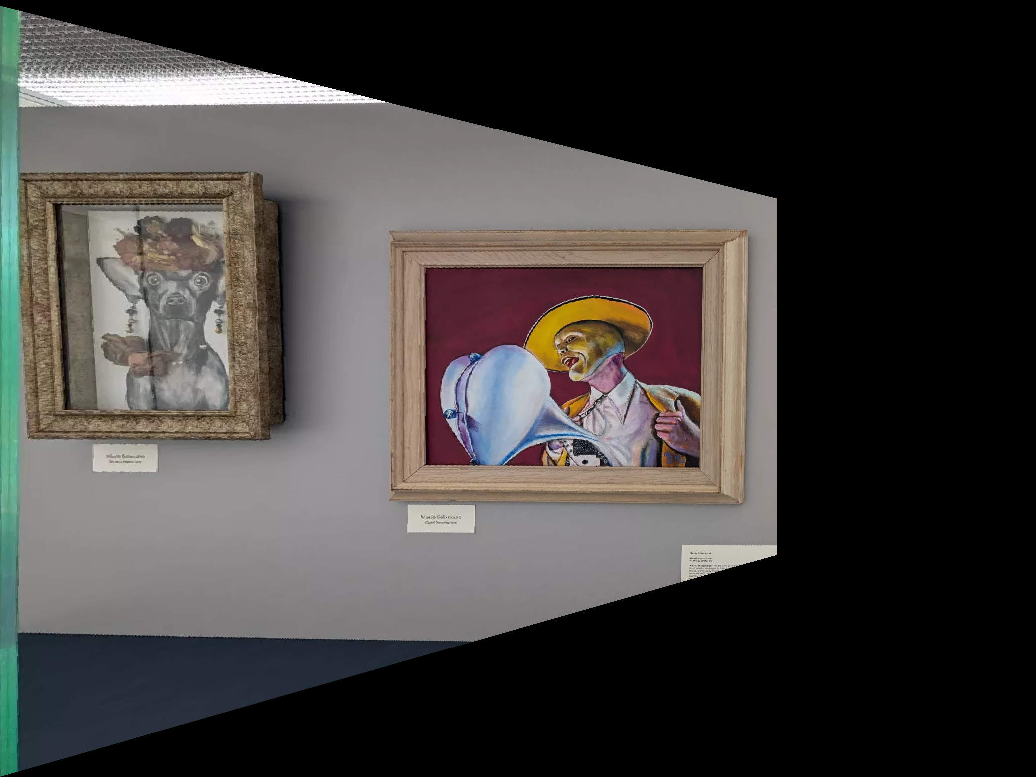
The rectification process involved defining corresponding points between the distorted rectangle and a target rectangle in the source image. (we picked points that define a rectangle when defining correspondences). As we can see in both images above, the distorted (due to perspective) rectangle has been rectified to a rectangle
Part 4A: Blend the Images into a Mosaic
In this final step, we blended the two images into a mosaic using the warped images - we also see if naive blending works well.
If naive blending wasn't working well, we tried to create a seamless mosaic by implementing a sophisticated blending technique that accounts for the overlap between the warped images. Our method involves the following key steps:
- Create binary masks for each image to identify non-black pixels.
- Identify the overlapping region between the two images.
- Generate weight matrices for each image using distance transforms. This assigns higher weights to pixels farther from the edge of each image.
- Normalize the weights in the overlapping region to ensure a smooth transition.
- Apply the weights to each image and combine them.
- Use the masks to fill in non-overlapping regions with the original image content.
This approach, which utilizes distance-based weighting, ensures a gradual and natural blend in the overlapping areas while preserving the original image content in non-overlapping regions. The result is a seamless mosaic that smoothly transitions between the input images.

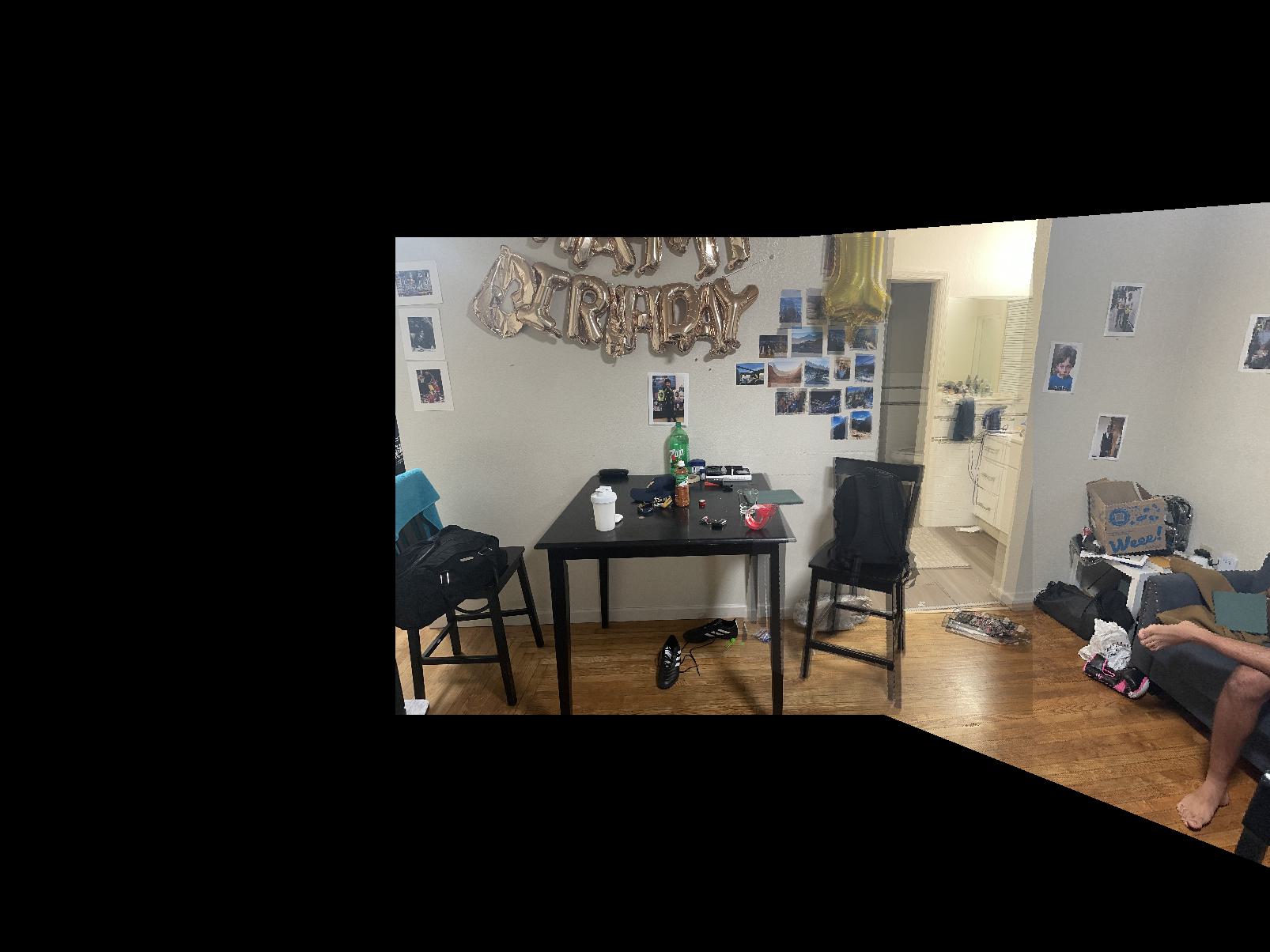

The image on the left has some artifacts (can be seen by looking closely at area near bathroom) which we can resolve by using alpha blending. The image on the right demonstrates the result of our blending technique, showing a smooth transition between the warped images and creating a cohesive panoramic view.
Part B: Automatic Feature Detection and Matching
Corner Detection
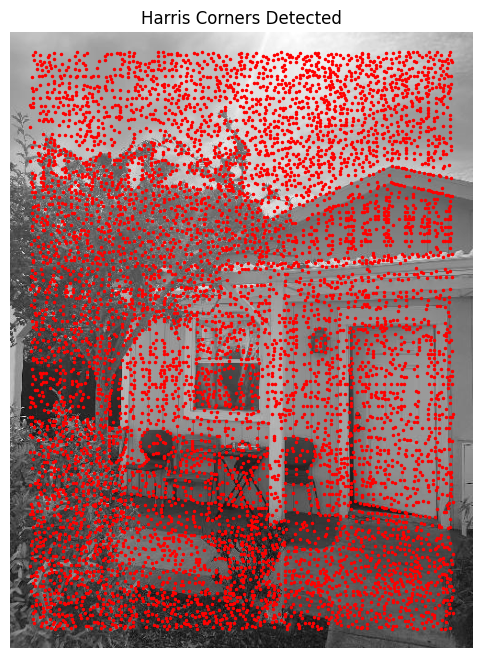
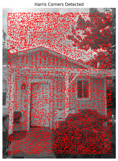
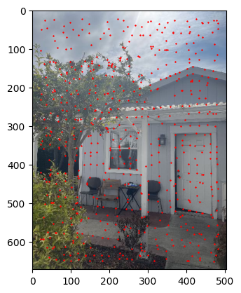
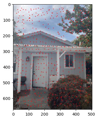
Implementation of Harris Corner Detection with Adaptive Non-Maximum Suppression (ANMS) to select 600 points.
Approach
The corner detection process involves:
- Using Harris corner detection algorithm to get scores h for each pixel
- Extracting scores into a vector: scores = h[corners[:, 0], corners[:, 1]]
- Implementing ANMS to identify strongest corners while maintaining even distribution
- Calculating pairwise distances using dist2()
- Using numpy broadcasting for f(x_i) < c_robust * f(x_j) comparison
- Creating masked distances and calculating minimum radii
- Sorting corners by decreasing radii and selecting best 600 corners
Feature Descriptors
Approach
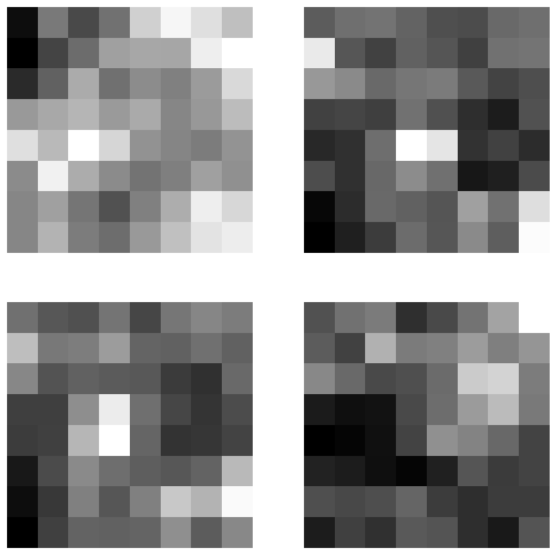
For each corner in points obtained from ANMS:
- Extract 40x40 region feature around the point from original color image
- Resize to 8x8 using skimage.transform.resize
- Normalize by subtracting mean and dividing by standard deviation for each channel
- Flatten and stack into matrix
Feature Matching
Approach
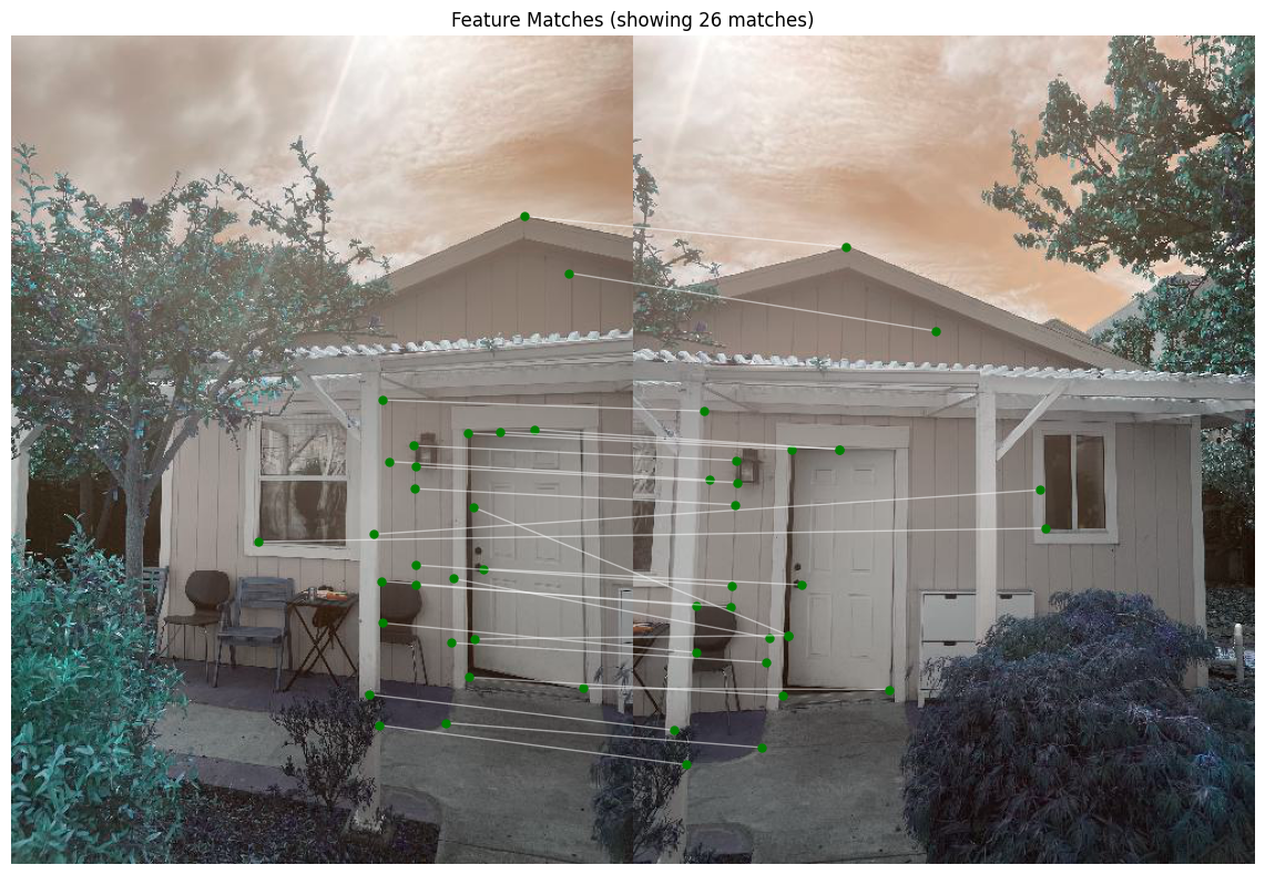
The matching process involves:
- Calculate pairwise differences between feature descriptors
- Compute sum-squared differences (SSD)
- Calculate Lowe scores using 2-NN distances
- Filter matches using threshold
- Pair corresponding features between images
Random Sample Consensus (RANSAC)
Approach
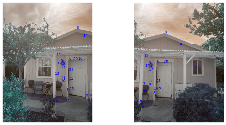
RANSAC implementation steps:
- Sample four points without replacement
- Compute homography using sampled points
- Transform all source points
- Calculate Euclidean distances to targets
- Identify inliers within threshold
- Update best set when more inliers found
Autostitched Mosaics
Results
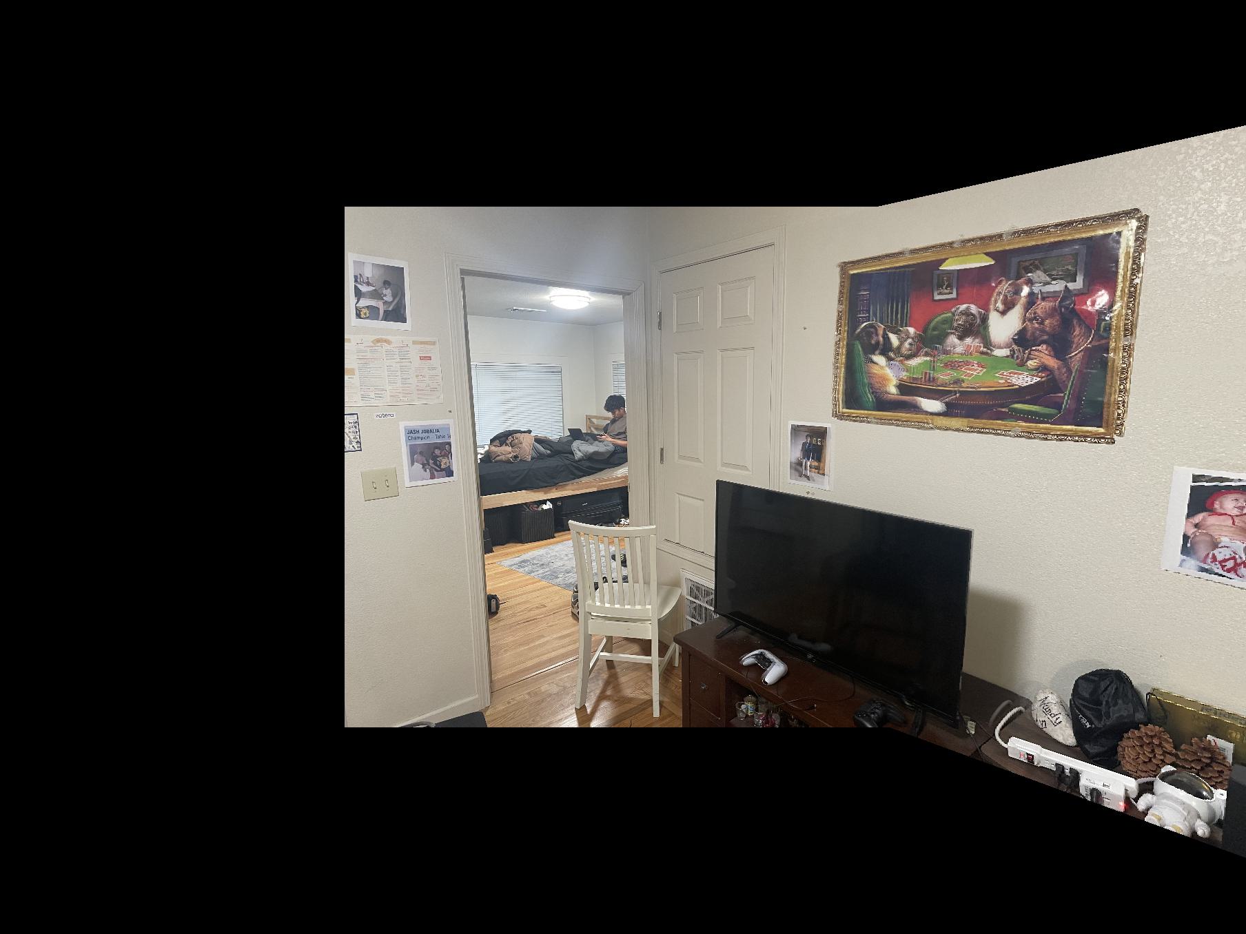
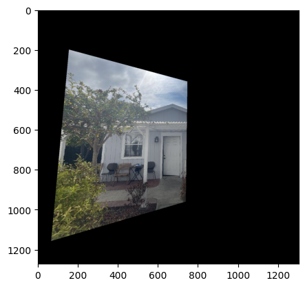
Comparison between manual and automatic stitching:

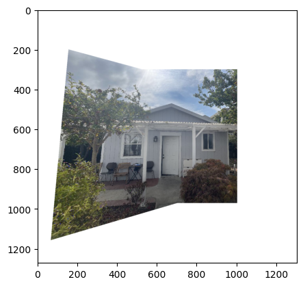

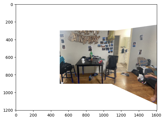

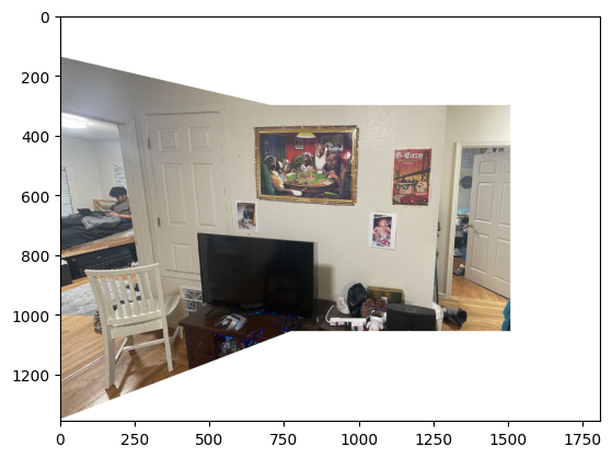
Key observations:
- Slightly less accurate than manual correspondences for some feature matches but much more efficient
- Limited control over feature selection
- Some misalignments in specific areas (chairs, walls, windows)
Reflection
Key insights from the project:
- Understanding homography matrix transformations and chaining
- Implementing efficient feature descriptor matching using broadcasting
- Visualizing algorithm-chosen features versus human-chosen features
- Comparing automatic versus manual stitching results
Overall this project was a great learning experience and helped me really unpack homographies, warping between geometries and how we can use basic math to achieve a task that sounds so impossible.